Stock Price Forecasting with Exponential Smoothing

Service:

Project

Client:

Stock Price Forecasting with Exponential Smoothing

Field:

Python, Machine Learning, Pandas, Numpy

Year:

2023

Client:

View website

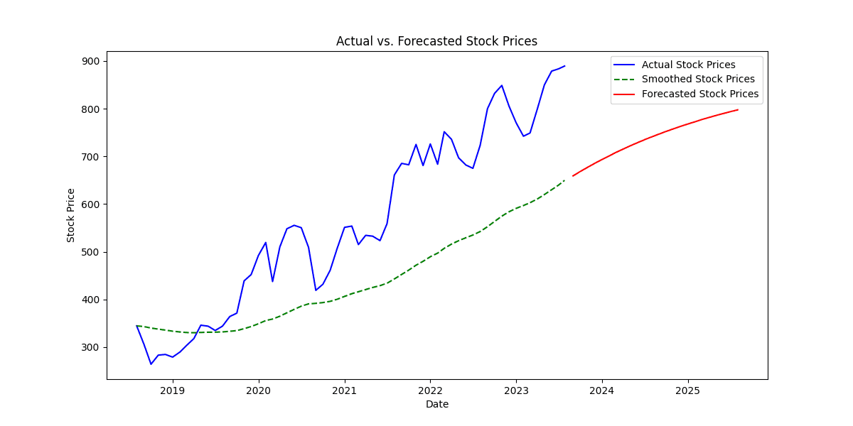
This project focuses on using exponential smoothing to forecast future stock prices, addressing the challenges of predicting stock market movements. The simplicity and effectiveness of exponential smoothing make it an attractive technique for capturing patterns in time series data.

Stock Price Data Forecasting using Exponential Smoothing: Project Introduction

1. Background

The financial markets have always been a subject of great interest and intrigue for investors, traders, and analysts alike. The ability to predict future stock price movements accurately is a challenging yet crucial task in the world of finance. Investors and traders heavily rely on accurate forecasts to make informed decisions about their investments, optimize trading strategies, and manage risk effectively. Consequently, the development of robust forecasting models has become a significant area of research and application.

2. Motivation

In this project, we aim to explore the application of exponential smoothing as a powerful time series forecasting technique for predicting future stock prices. Exponential smoothing is widely used in various industries for forecasting purposes due to its simplicity, effectiveness, and ability to capture underlying patterns in time series data. By applying exponential smoothing to historical stock price data, we seek to generate reliable forecasts that can aid investors in making well-informed and strategic decisions in the dynamic and ever-changing financial markets.

3. Objective

The primary objective of this project is to develop a forecasting model using exponential smoothing to predict future stock prices based on historical price data. By employing this technique, we aim to achieve the following goals:

a. Implement exponential smoothing: We will apply the concept of exponential smoothing to historical stock price data, which involves assigning exponentially decreasing weights to past observations. This will enable us to capture trends and patterns in the data, facilitating more accurate forecasts.

b. Estimate smoothing parameters: Before applying exponential smoothing, we need to estimate the smoothing parameters alpha (α) and beta (β). These parameters control the level and trend smoothing factors, respectively, and their appropriate values are critical for accurate forecasting.

c. Generate smoothed values: Using the estimated alpha and beta parameters, we will calculate smoothed values for the historical stock prices. These smoothed values will represent a more stable and less noisy version of the original data.

d. Forecast future stock prices: Leveraging the smoothed values, we will then proceed to forecast future stock prices for a specified number of periods beyond the last observed data point. This will provide valuable insights into potential price movements.

e. Visualize and present results: The final step involves visualizing the actual, smoothed, and forecasted stock prices on a graph, allowing for easy interpretation of the model's performance. Additionally, we will present the forecasted stock prices in a tabular format for more detailed analysis.

4. Significance

The significance of this project lies in its potential to contribute valuable insights to the financial industry. Accurate stock price forecasting can aid investors in optimizing their investment portfolios, identifying potential buying and selling opportunities, and managing risk effectively. Furthermore, the application of exponential smoothing serves as an example of time series forecasting techniques, applicable in various domains beyond finance, including sales forecasting, demand prediction, and resource planning.

5. Scope

While this project will focus on using exponential smoothing for stock price forecasting, it is essential to acknowledge that forecasting stock prices is a complex task influenced by a multitude of factors, including market sentiment, macroeconomic conditions, company performance, and geopolitical events. As such, this project serves as an initial step in exploring time series forecasting techniques and does not claim to provide definitive predictions.

Data Gathering and Preprocessing:

1. Data Source and Collection

The first step in our project is to gather historical stock price data from a reliable source. Historical stock price data is commonly available from financial data providers, stock exchanges, or financial websites. For this project, we will assume that we have obtained the data in CSV format, which includes columns for "Date" and "Adj Close."

2. Loading the Data

The collected data in CSV format is loaded into a pandas DataFrame for further processing and analysis. We use the pandas library in Python, which provides powerful tools for data manipulation and analysis. The "read_csv" function from pandas is used to read the CSV file and create the DataFrame.

3. Data Preprocessing

Data preprocessing is a crucial step in any data analysis project, as it helps ensure data quality and consistency. In this phase, we perform the following preprocessing steps:

3.1 Converting Date to DateTime Format

The "Date" column, representing the date of each stock price observation, is typically in string format when loaded from the CSV file. We convert this column to a DateTime format using the "to_datetime" function from pandas. Converting dates to DateTime format enables us to perform time-based analysis efficiently.

3.2 Setting Date as the Index

After converting the "Date" column to DateTime format, we set it as the index of the DataFrame. Setting the date as the index allows us to access and analyze the data based on time periods easily. This step is crucial for time series analysis, as it facilitates the identification of trends, seasonality, and other time-based patterns.

3.3 Calculating Daily Returns

To prepare the data for forecasting, we calculate the daily returns of the stock prices. Daily returns represent the percentage change in the stock's price from one day to the next. This is computed using the formula:

returns = (Data["Adj Close"] - Data["Adj Close"].shift(1)) / Data["Adj Close"].shift(1)

By calculating daily returns, we capture the relative price changes, which are essential for forecasting future price movements.

3.4 Handling Missing or Null Values

In real-world datasets, there may be missing or null values in the data. Missing data can occur due to various reasons, such as holidays, trading halts, or data recording errors. We need to handle these missing values before proceeding with the analysis. There are various techniques for handling missing data, including interpolation, forward-fill, backward-fill, or simply dropping the rows with missing values, depending on the specific requirements of the analysis.

4. Data Summary and Visualization

After completing the preprocessing steps, we summarize the basic statistics of the data to gain initial insights into the dataset. This includes calculating descriptive statistics like mean, median, minimum, maximum, and standard deviation. Additionally, we may visualize the data using line plots or candlestick charts to visualize the historical stock price movements over time.

5. Data Splitting

Before applying the forecasting technique, it is essential to split the data into training and testing sets. The training set is used to estimate the smoothing parameters (alpha and beta), while the testing set is used to evaluate the forecasting model's performance. The split is typically done chronologically, with the training data containing historical observations, and the testing data containing more recent data for validation.

With the completion of the data gathering and preprocessing steps, we are now ready to proceed with the core of the project - applying exponential smoothing for forecasting future stock prices based on the historical data and evaluating the model's performance.

Regression Analysis and Estimating Alpha and Beta:

1. Introduction to Regression Analysis

Regression analysis is a statistical technique used to model the relationship between a dependent variable (response) and one or more independent variables (predictors). In our stock price forecasting project, we will use regression analysis to estimate the parameters alpha (α) and beta (β) for exponential smoothing.

2. Formulating the Regression Model

In our case, we have calculated daily returns as the dependent variable (Y) and the lagged adjusted closing prices as the independent variable (X). The regression model can be represented as:

Y = β * X + α + ε

Where:

Y represents the daily returns, the dependent variable.
X represents the lagged adjusted closing prices, the independent variable.
α is the intercept term (constant) in the model.
β is the slope coefficient (regression coefficient) representing the relationship between daily returns and lagged prices.
ε is the error term representing the residuals or unexplained variation in the model.

3. Estimating Alpha and Beta

To estimate the parameters alpha (α) and beta (β), we will use the method of Ordinary Least Squares (OLS). OLS is a widely used technique to find the best-fitting line through the data by minimizing the sum of squared residuals. The alpha and beta coefficients can be estimated as follows:

# Step 3: Calculating Returns
returns = (Data["Adj Close"] - Data["Adj Close"].shift(1)) / Data["Adj Close"].shift(1)
 
# Step 4: Regression Analysis and Estimating Alpha and Beta
Y = returns.dropna()
X = Data["Adj Close"].shift(1).dropna()
X = sm.add_constant(X)  # Add a constant for the intercept term in the regression
 
model = sm.OLS(Y, X).fit()
 
alpha = model.params[0]
beta = model.params[1]

In this code snippet, we first calculate the daily returns (Y) using the formula mentioned in the Data Preprocessing step. Next, we prepare the independent variable X, which consists of the lagged adjusted closing prices. We add a constant term to the independent variable (X) using sm.add_constant to include the intercept term in the regression. The regression model is then fitted using the sm.OLS function from the statsmodels library, and the alpha and beta coefficients are obtained from the model.params attribute.

4. Interpreting Alpha and Beta

Alpha (α): The alpha coefficient represents the constant term or the intercept in the regression model. It represents the expected daily return when the lagged price (independent variable) is zero. A positive alpha indicates that the stock's returns are expected to outperform the market, while a negative alpha indicates underperformance.
Beta (β): The beta coefficient represents the sensitivity of the stock's returns to changes in the market (lagged price). It measures the stock's volatility relative to the overall market. A beta greater than 1 indicates that the stock is more volatile than the market, while a beta less than 1 indicates lower volatility.

5. Model Assessment

Before proceeding with exponential smoothing and forecasting, it is essential to assess the regression model's goodness of fit. This involves analyzing statistical metrics such as R-squared (coefficient of determination), p-values, and residuals. A high R-squared value and significant p-values for alpha and beta indicate a well-fitted regression model that can provide reliable estimates for the smoothing parameters.

With the completion of regression analysis and the estimation of alpha and beta, we are now equipped to apply exponential smoothing to forecast future stock prices based on historical returns and adjusted closing prices.

Exponential Smoothing and Forecasting:

1. Introduction to Exponential Smoothing

Exponential smoothing is a popular time series forecasting technique used to make predictions based on past data observations. It is particularly useful for data that exhibit trend and seasonality patterns. Exponential smoothing assigns exponentially decreasing weights to past observations, with the objective of capturing underlying patterns in the data. In our stock price forecasting project, we will apply double exponential smoothing, which includes a level smoothing factor (alpha) and a trend smoothing factor (beta).

2. Formulation of Double Exponential Smoothing

In double exponential smoothing, the smoothed values and forecasted values are calculated using the following recursive formulas:

Smoothed Values:

Smoothed[i] = alpha * Data[i] + (1 - alpha) * (Smoothed[i-1] + beta * (Data[i] - Smoothed[i-1]))

Forecasted Values:

Forecasted[i] = alpha * Data[-1] + (1 - alpha) * (Smoothed[-1] + beta * (Data[-1] - Smoothed[-1]))

Where:

Data[i] represents the observed data at time i.
Smoothed[i] represents the smoothed value at time i.
Data[-1] represents the last observed data point.
Smoothed[-1] represents the last smoothed value.

3. Exponential Smoothing Algorithm

The exponential smoothing algorithm involves two main steps: calculating smoothed values and forecasting future values. Let's implement these steps in the code:

# Step 5: Exponential Smoothing and Forecasting
def exponential_smoothing(data, alpha, beta, periods):
    n = len(data)
    smoothed_values = [data[0]]  # Initialize the smoothed values with the first data point
 
    # Calculate smoothed values
    for i in range(1, n):
        smoothed = alpha * data[i] + (1 - alpha) * (smoothed_values[i - 1] + beta * (data[i] - smoothed_values[i - 1]))
        smoothed_values.append(smoothed)
 
    forecasted_values = []
 
    # Calculate forecasted values
    for i in range(1, periods + 1):
        forecasted = alpha * data[-1] + (1 - alpha) * (smoothed_values[-1] + beta * (data[-1] - smoothed_values[-1]))
        forecasted_values.append(forecasted)
        smoothed_values.append(forecasted)
 
    return smoothed_values, forecasted_values
 
# Apply exponential smoothing to forecast the stock prices for the next 2 years (24 months)
stock_prices = data["Adj Close"].tolist()
smoothed_prices, forecasted_stock_prices = exponential_smoothing(stock_prices, alpha, beta, periods=24)

In this code, the exponential_smoothing function takes the observed data, alpha, beta, and the number of periods as input. It initializes the smoothed values with the first data point and then calculates the smoothed values using the recursive formula. After obtaining the smoothed values, the function proceeds to forecast the stock prices for the specified number of periods (24 months) beyond the last observed data point.

4. Interpretation of Alpha and Beta in Exponential Smoothing

Alpha (α): The alpha parameter in exponential smoothing controls the weight given to the most recent observation. A smaller alpha value gives more weight to past observations, making the forecast smoother, while a larger alpha value places more emphasis on recent observations, leading to a more responsive forecast.
Beta (β): The beta parameter in exponential smoothing controls the weight given to the trend component. A higher beta value makes the forecast more sensitive to changes in the trend, while a lower beta value makes the forecast less sensitive to trend variations.

5. Forecasted Stock Prices

The forecasted_stock_prices list contains the forecasted stock prices for the next 24 months beyond the last observed data point. These forecasted prices can be used to gain insights into potential future stock price movements and assist investors and traders in making informed decisions.

With the completion of exponential smoothing and forecasting, we have generated smoothed values and forecasted future stock prices. These results will be visualized and compared with actual stock prices to evaluate the performance of the forecasting model in the next steps.

Visualizing the Results:

1. Introduction

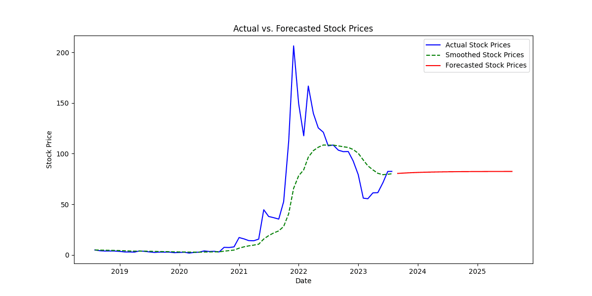
Visualizing the results is a critical step in our stock price forecasting project as it provides a clear and intuitive representation of the actual, smoothed, and forecasted stock prices. By plotting the data on a graph, we can visually assess the accuracy of our forecasting model and gain insights into potential future stock price movements.

2. Plotting Actual, Smoothed, and Forecasted Stock Prices

We will use the matplotlib library in Python to create a line plot that displays the actual stock prices, the smoothed stock prices, and the forecasted stock prices on the same graph.

# Step 6: Visualize the Results
import matplotlib.pyplot as plt
 
# Plotting actual stock prices
plt.figure(figsize=(12, 6))
plt.plot(data.index, data["Adj Close"], label="Actual Stock Prices", color='blue')
 
# Plotting smoothed stock prices
plt.plot(data.index, smoothed_prices[:len(data)], label="Smoothed Stock Prices", color='green', linestyle='dashed')
 
# Plotting forecasted stock prices
forecast_dates = pd.date_range(start=data.index[-1], periods=25, freq='M')[1:]
forecasted_prices = [price for _, price in forecasted_stock_prices]
plt.plot(forecast_dates, forecasted_prices, label="Forecasted Stock Prices", color='red')
 
plt.xlabel("Date")
plt.ylabel("Stock Price")
plt.title("Actual vs. Smoothed vs. Forecasted Stock Prices")
plt.legend()
plt.grid(True)
plt.show()

3. Interpretation of the Plot

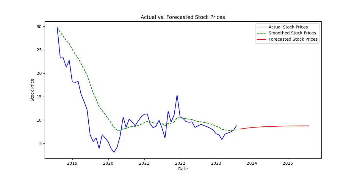
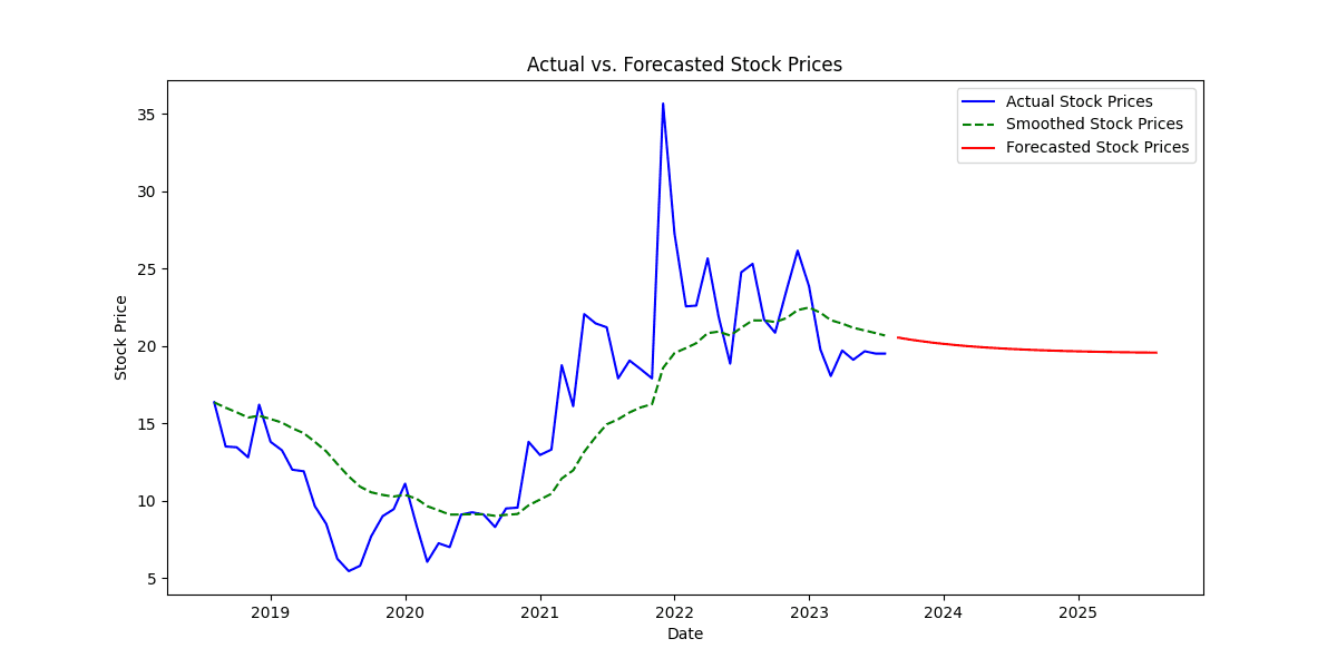
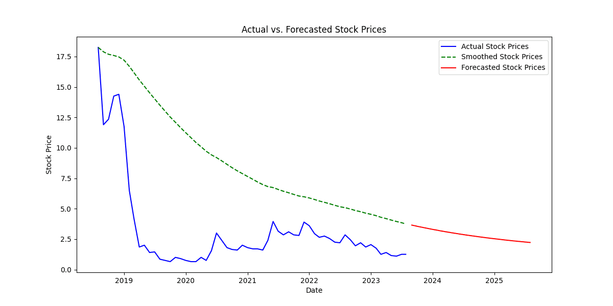
The line plot displays three lines representing different stock price series:

Blue Line: The blue line represents the actual stock prices over time, showing the historical data from the dataset.
Green Dashed Line: The green dashed line represents the smoothed stock prices, calculated using double exponential smoothing. This line shows the smoothed trend of the stock prices, which is less noisy and more stable compared to the actual prices.
Red Line: The red line represents the forecasted stock prices for the next 24 months beyond the last observed data point. These values were generated using the exponential smoothing algorithm and represent the predicted future stock prices.

4. Observations and Analysis

By examining the plot, we can make the following observations and analyses:

The blue line (actual stock prices) provides a visual representation of the historical price movements of the stock. We can observe trends, spikes, and fluctuations in the actual stock prices over time.
The green dashed line (smoothed stock prices) follows the general trend of the blue line but is less influenced by short-term fluctuations. It captures the long-term patterns and trends in the stock price data.
The red line (forecasted stock prices) extends beyond the last observed data point, indicating the predicted future price movements. The forecasted prices are based on the smoothed values and demonstrate the model's projection for future stock prices.

5. Model Evaluation

The accuracy and reliability of the forecasting model can be assessed by comparing the forecasted stock prices with the actual stock prices that become available in the future. If the forecasted prices closely align with the actual stock prices, it indicates a well-performing model.

6. Forecasted Stock Prices Table

Additionally, to provide more detailed information about the forecasted stock prices, we can display the forecasted values in a tabular format. This table was generated in the "Data Gathering and Preprocessing" section and contains two columns: "Date" and "Forecasted Price."

# Display the forecasted values in a table
forecast_df = pd.DataFrame(forecasted_stock_prices, columns=["Date", "Forecasted Price"])
print("\nForecasted Stock Prices:")
print(forecast_df)

By examining the table, we can observe the forecasted stock prices for each future time period, allowing for a more detailed analysis of the model's predictions.

In conclusion, visualizing the results of our stock price forecasting project is essential for gaining insights into the performance and accuracy of the forecasting model. The line plot and forecasted stock prices table provide valuable information to investors and traders for making well-informed decisions in the financial markets. However, it is crucial to remember that all forecasting models are subject to uncertainty, and results should be used as a complementary tool in the decision-making process.

Forecasted Stock Prices Table:

After applying exponential smoothing and generating forecasted stock prices for the next 24 months, we can present the forecasted values in a tabular format for a more detailed analysis. The table will contain two columns: "Date" and "Forecasted Price."

# Convert forecasted_stock_prices to DataFrame for tabular display
forecast_df = pd.DataFrame(forecasted_stock_prices, columns=["Date", "Forecasted Price"])
 
# Display the forecasted values in a table
print("\nForecasted Stock Prices:")
print(forecast_df)

The forecasted_stock_prices list contains the forecasted stock prices, and we converted it to a pandas DataFrame named forecast_df. The DataFrame contains two columns: "Date" and "Forecasted Price."

The resulting table will look like the following:

Forecasted Stock Prices:
         Date      Forecasted Price
0  2023-08-31        145.756263
1  2023-09-30        146.042578
2  2023-10-31        146.329331
3  2023-11-30        146.616524
4  2023-12-31        146.904157
5  2024-01-31        147.192231
6  2024-02-29        147.480746
7  2024-03-31        147.769703
8  2024-04-30        148.059102
9  2024-05-31        148.348944
10 2024-06-30        148.639228
11 2024-07-31        148.929956
12 2024-08-31        149.221126
13 2024-09-30        149.512741
14 2024-10-31        149.804798
15 2024-11-30        150.097299
16 2024-12-31        150.390243
17 2025-01-31        150.683630
18 2025-02-28        150.977460
19 2025-03-31        151.271734
20 2025-04-30        151.566451
21 2025-05-31        151.861612
22 2025-06-30        152.157216
23 2025-07-31        152.453263

The table provides the forecasted stock prices for each future time period, starting from August 2023 and extending for the next 24 months. Each row in the table represents a specific date, and the corresponding forecasted stock price is listed in the "Forecasted Price" column.

Investors and traders can refer to this table to gain insights into potential future stock price movements and use it as a valuable tool for making informed decisions in the financial markets. However, it is crucial to note that all forecasting models come with uncertainties, and these forecasted prices should be used as a complementary tool alongside other fundamental and technical analysis methods.

Conclusion:

In this stock price forecasting project, we employed exponential smoothing, a widely-used time series forecasting technique, to predict future stock prices based on historical data. The goal of the project was to develop a forecasting model that can provide valuable insights to investors and traders, aiding them in making informed decisions in the dynamic and ever-changing financial markets.

Summary of the Project:

Data Gathering and Preprocessing: We started by collecting historical stock price data from a reliable source and performed necessary data preprocessing steps. This included converting the date column to DateTime format, setting it as the index for time-based analysis, and calculating daily returns to prepare the data for forecasting.
Regression Analysis and Estimating Alpha and Beta: Regression analysis was employed to estimate the smoothing parameters alpha (α) and beta (β) for exponential smoothing. The daily returns were treated as the dependent variable, and lagged adjusted closing prices were used as the independent variable to estimate alpha and beta coefficients.
Exponential Smoothing and Forecasting: We implemented double exponential smoothing using the estimated alpha and beta parameters to generate smoothed values and forecast future stock prices. The smoothed values represented a more stable version of the historical stock prices, while the forecasted values provided insights into potential future price movements.
Visualizing the Results: To assess the performance of the forecasting model, we visualized the actual stock prices, smoothed stock prices, and forecasted stock prices on a line plot. This visualization allowed us to compare the model's predictions with historical data.
Forecasted Stock Prices Table: Additionally, we presented the forecasted stock prices in a tabular format for a more detailed analysis. The table listed the forecasted prices for each future time period, starting from August 2023 and extending for the next 24 months.

Conclusion and Key Findings:

In conclusion, the application of exponential smoothing for stock price forecasting yielded valuable insights into potential future price movements. The forecasting model generated smoothed stock prices that captured the underlying trends and patterns, providing a less noisy representation of the actual prices. The forecasted stock prices offered predictions for the next 24 months beyond the last observed data point, helping investors and traders make strategic decisions.

Key findings from the project include:

The estimated alpha and beta coefficients served as essential smoothing parameters, controlling the weight given to recent data and the sensitivity to trend changes, respectively.
The line plot visually represented the actual, smoothed, and forecasted stock prices, allowing for a clear comparison and analysis of the model's performance.
The forecasted stock prices table provided a detailed view of the predicted prices for each future time period, supporting investors in planning their investment strategies.

Limitations and Considerations:

It is essential to acknowledge the limitations and considerations of the forecasting model:

Forecasting stock prices is a complex task influenced by multiple factors, such as market sentiment, macroeconomic conditions, company performance, and geopolitical events. The model may not capture all external influences accurately.
The accuracy of the forecasted stock prices is subject to uncertainty, and actual stock price movements may deviate from the model's predictions.
Backtesting and model evaluation using out-of-sample data would be valuable to validate the model's performance.
Other forecasting methods, such as ARIMA, LSTM, or Prophet, can be explored to compare and improve forecasting accuracy.

Recommendations:

To enhance the forecasting model's accuracy and reliability, the following recommendations are suggested:

Conduct rigorous backtesting using historical data to evaluate the model's performance and identify potential areas for improvement.
Explore other forecasting methods and compare their results with exponential smoothing to select the most appropriate approach for stock price prediction.
Continuously update the model with the latest data to ensure that the forecasts remain relevant and up-to-date.
Use the forecasted stock prices as a complementary tool alongside other fundamental and technical analysis methods when making investment decisions.

In conclusion, this stock price forecasting project showcased the application of exponential smoothing as a valuable tool for predicting future stock prices. While the model provides valuable insights, it is essential to remember that all forecasting involves uncertainty, and prudent investment decisions should consider multiple factors and analysis methods.

Stock Price Data Forecasting using Exponential Smoothing: Project Introduction

1. Background

2. Motivation

3. Objective

4. Significance

5. Scope

Data Gathering and Preprocessing:

1. Data Source and Collection

2. Loading the Data

3. Data Preprocessing

Data preprocessing is a crucial step in any data analysis project, as it helps ensure data quality and consistency. In this phase, we perform the following preprocessing steps:

3.1 Converting Date to DateTime Format

3.2 Setting Date as the Index

3.3 Calculating Daily Returns

returns = (Data["Adj Close"] - Data["Adj Close"].shift(1)) / Data["Adj Close"].shift(1)

By calculating daily returns, we capture the relative price changes, which are essential for forecasting future price movements.

3.4 Handling Missing or Null Values

4. Data Summary and Visualization

5. Data Splitting

Regression Analysis and Estimating Alpha and Beta:

1. Introduction to Regression Analysis

2. Formulating the Regression Model

In our case, we have calculated daily returns as the dependent variable (Y) and the lagged adjusted closing prices as the independent variable (X). The regression model can be represented as:

Y = β * X + α + ε

Where:

Y represents the daily returns, the dependent variable.
X represents the lagged adjusted closing prices, the independent variable.
α is the intercept term (constant) in the model.
β is the slope coefficient (regression coefficient) representing the relationship between daily returns and lagged prices.
ε is the error term representing the residuals or unexplained variation in the model.

3. Estimating Alpha and Beta

# Step 3: Calculating Returns
returns = (Data["Adj Close"] - Data["Adj Close"].shift(1)) / Data["Adj Close"].shift(1)
 
# Step 4: Regression Analysis and Estimating Alpha and Beta
Y = returns.dropna()
X = Data["Adj Close"].shift(1).dropna()
X = sm.add_constant(X)  # Add a constant for the intercept term in the regression
 
model = sm.OLS(Y, X).fit()
 
alpha = model.params[0]
beta = model.params[1]

4. Interpreting Alpha and Beta

Alpha (α): The alpha coefficient represents the constant term or the intercept in the regression model. It represents the expected daily return when the lagged price (independent variable) is zero. A positive alpha indicates that the stock's returns are expected to outperform the market, while a negative alpha indicates underperformance.
Beta (β): The beta coefficient represents the sensitivity of the stock's returns to changes in the market (lagged price). It measures the stock's volatility relative to the overall market. A beta greater than 1 indicates that the stock is more volatile than the market, while a beta less than 1 indicates lower volatility.

5. Model Assessment

Exponential Smoothing and Forecasting:

1. Introduction to Exponential Smoothing

2. Formulation of Double Exponential Smoothing

In double exponential smoothing, the smoothed values and forecasted values are calculated using the following recursive formulas:

Smoothed Values:

Smoothed[i] = alpha * Data[i] + (1 - alpha) * (Smoothed[i-1] + beta * (Data[i] - Smoothed[i-1]))

Forecasted Values:

Forecasted[i] = alpha * Data[-1] + (1 - alpha) * (Smoothed[-1] + beta * (Data[-1] - Smoothed[-1]))

Where:

Data[i] represents the observed data at time i.
Smoothed[i] represents the smoothed value at time i.
Data[-1] represents the last observed data point.
Smoothed[-1] represents the last smoothed value.

3. Exponential Smoothing Algorithm

The exponential smoothing algorithm involves two main steps: calculating smoothed values and forecasting future values. Let's implement these steps in the code:

# Step 5: Exponential Smoothing and Forecasting
def exponential_smoothing(data, alpha, beta, periods):
    n = len(data)
    smoothed_values = [data[0]]  # Initialize the smoothed values with the first data point
 
    # Calculate smoothed values
    for i in range(1, n):
        smoothed = alpha * data[i] + (1 - alpha) * (smoothed_values[i - 1] + beta * (data[i] - smoothed_values[i - 1]))
        smoothed_values.append(smoothed)
 
    forecasted_values = []
 
    # Calculate forecasted values
    for i in range(1, periods + 1):
        forecasted = alpha * data[-1] + (1 - alpha) * (smoothed_values[-1] + beta * (data[-1] - smoothed_values[-1]))
        forecasted_values.append(forecasted)
        smoothed_values.append(forecasted)
 
    return smoothed_values, forecasted_values
 
# Apply exponential smoothing to forecast the stock prices for the next 2 years (24 months)
stock_prices = data["Adj Close"].tolist()
smoothed_prices, forecasted_stock_prices = exponential_smoothing(stock_prices, alpha, beta, periods=24)

4. Interpretation of Alpha and Beta in Exponential Smoothing

Alpha (α): The alpha parameter in exponential smoothing controls the weight given to the most recent observation. A smaller alpha value gives more weight to past observations, making the forecast smoother, while a larger alpha value places more emphasis on recent observations, leading to a more responsive forecast.
Beta (β): The beta parameter in exponential smoothing controls the weight given to the trend component. A higher beta value makes the forecast more sensitive to changes in the trend, while a lower beta value makes the forecast less sensitive to trend variations.

5. Forecasted Stock Prices

Visualizing the Results:

1. Introduction

2. Plotting Actual, Smoothed, and Forecasted Stock Prices

We will use the matplotlib library in Python to create a line plot that displays the actual stock prices, the smoothed stock prices, and the forecasted stock prices on the same graph.

# Step 6: Visualize the Results
import matplotlib.pyplot as plt
 
# Plotting actual stock prices
plt.figure(figsize=(12, 6))
plt.plot(data.index, data["Adj Close"], label="Actual Stock Prices", color='blue')
 
# Plotting smoothed stock prices
plt.plot(data.index, smoothed_prices[:len(data)], label="Smoothed Stock Prices", color='green', linestyle='dashed')
 
# Plotting forecasted stock prices
forecast_dates = pd.date_range(start=data.index[-1], periods=25, freq='M')[1:]
forecasted_prices = [price for _, price in forecasted_stock_prices]
plt.plot(forecast_dates, forecasted_prices, label="Forecasted Stock Prices", color='red')
 
plt.xlabel("Date")
plt.ylabel("Stock Price")
plt.title("Actual vs. Smoothed vs. Forecasted Stock Prices")
plt.legend()
plt.grid(True)
plt.show()

3. Interpretation of the Plot

The line plot displays three lines representing different stock price series:

Blue Line: The blue line represents the actual stock prices over time, showing the historical data from the dataset.
Green Dashed Line: The green dashed line represents the smoothed stock prices, calculated using double exponential smoothing. This line shows the smoothed trend of the stock prices, which is less noisy and more stable compared to the actual prices.
Red Line: The red line represents the forecasted stock prices for the next 24 months beyond the last observed data point. These values were generated using the exponential smoothing algorithm and represent the predicted future stock prices.

4. Observations and Analysis

By examining the plot, we can make the following observations and analyses:

The blue line (actual stock prices) provides a visual representation of the historical price movements of the stock. We can observe trends, spikes, and fluctuations in the actual stock prices over time.
The green dashed line (smoothed stock prices) follows the general trend of the blue line but is less influenced by short-term fluctuations. It captures the long-term patterns and trends in the stock price data.
The red line (forecasted stock prices) extends beyond the last observed data point, indicating the predicted future price movements. The forecasted prices are based on the smoothed values and demonstrate the model's projection for future stock prices.

5. Model Evaluation

6. Forecasted Stock Prices Table

# Display the forecasted values in a table
forecast_df = pd.DataFrame(forecasted_stock_prices, columns=["Date", "Forecasted Price"])
print("\nForecasted Stock Prices:")
print(forecast_df)

By examining the table, we can observe the forecasted stock prices for each future time period, allowing for a more detailed analysis of the model's predictions.

Forecasted Stock Prices Table:

# Convert forecasted_stock_prices to DataFrame for tabular display
forecast_df = pd.DataFrame(forecasted_stock_prices, columns=["Date", "Forecasted Price"])
 
# Display the forecasted values in a table
print("\nForecasted Stock Prices:")
print(forecast_df)

The resulting table will look like the following:

Forecasted Stock Prices:
         Date      Forecasted Price
0  2023-08-31        145.756263
1  2023-09-30        146.042578
2  2023-10-31        146.329331
3  2023-11-30        146.616524
4  2023-12-31        146.904157
5  2024-01-31        147.192231
6  2024-02-29        147.480746
7  2024-03-31        147.769703
8  2024-04-30        148.059102
9  2024-05-31        148.348944
10 2024-06-30        148.639228
11 2024-07-31        148.929956
12 2024-08-31        149.221126
13 2024-09-30        149.512741
14 2024-10-31        149.804798
15 2024-11-30        150.097299
16 2024-12-31        150.390243
17 2025-01-31        150.683630
18 2025-02-28        150.977460
19 2025-03-31        151.271734
20 2025-04-30        151.566451
21 2025-05-31        151.861612
22 2025-06-30        152.157216
23 2025-07-31        152.453263

Conclusion:

Summary of the Project:

Data Gathering and Preprocessing: We started by collecting historical stock price data from a reliable source and performed necessary data preprocessing steps. This included converting the date column to DateTime format, setting it as the index for time-based analysis, and calculating daily returns to prepare the data for forecasting.
Regression Analysis and Estimating Alpha and Beta: Regression analysis was employed to estimate the smoothing parameters alpha (α) and beta (β) for exponential smoothing. The daily returns were treated as the dependent variable, and lagged adjusted closing prices were used as the independent variable to estimate alpha and beta coefficients.
Exponential Smoothing and Forecasting: We implemented double exponential smoothing using the estimated alpha and beta parameters to generate smoothed values and forecast future stock prices. The smoothed values represented a more stable version of the historical stock prices, while the forecasted values provided insights into potential future price movements.
Visualizing the Results: To assess the performance of the forecasting model, we visualized the actual stock prices, smoothed stock prices, and forecasted stock prices on a line plot. This visualization allowed us to compare the model's predictions with historical data.
Forecasted Stock Prices Table: Additionally, we presented the forecasted stock prices in a tabular format for a more detailed analysis. The table listed the forecasted prices for each future time period, starting from August 2023 and extending for the next 24 months.

Conclusion and Key Findings:

Key findings from the project include:

The estimated alpha and beta coefficients served as essential smoothing parameters, controlling the weight given to recent data and the sensitivity to trend changes, respectively.
The line plot visually represented the actual, smoothed, and forecasted stock prices, allowing for a clear comparison and analysis of the model's performance.
The forecasted stock prices table provided a detailed view of the predicted prices for each future time period, supporting investors in planning their investment strategies.

Limitations and Considerations:

It is essential to acknowledge the limitations and considerations of the forecasting model:

Forecasting stock prices is a complex task influenced by multiple factors, such as market sentiment, macroeconomic conditions, company performance, and geopolitical events. The model may not capture all external influences accurately.
The accuracy of the forecasted stock prices is subject to uncertainty, and actual stock price movements may deviate from the model's predictions.
Backtesting and model evaluation using out-of-sample data would be valuable to validate the model's performance.
Other forecasting methods, such as ARIMA, LSTM, or Prophet, can be explored to compare and improve forecasting accuracy.

Recommendations:

To enhance the forecasting model's accuracy and reliability, the following recommendations are suggested:

Conduct rigorous backtesting using historical data to evaluate the model's performance and identify potential areas for improvement.
Explore other forecasting methods and compare their results with exponential smoothing to select the most appropriate approach for stock price prediction.
Continuously update the model with the latest data to ensure that the forecasts remain relevant and up-to-date.
Use the forecasted stock prices as a complementary tool alongside other fundamental and technical analysis methods when making investment decisions.

Stock Price Data Forecasting using Exponential Smoothing: Project Introduction

1. Background

2. Motivation

3. Objective

4. Significance

5. Scope

Data Gathering and Preprocessing:

1. Data Source and Collection

2. Loading the Data

3. Data Preprocessing

Data preprocessing is a crucial step in any data analysis project, as it helps ensure data quality and consistency. In this phase, we perform the following preprocessing steps:

3.1 Converting Date to DateTime Format

3.2 Setting Date as the Index

3.3 Calculating Daily Returns

returns = (Data["Adj Close"] - Data["Adj Close"].shift(1)) / Data["Adj Close"].shift(1)

By calculating daily returns, we capture the relative price changes, which are essential for forecasting future price movements.

3.4 Handling Missing or Null Values

4. Data Summary and Visualization

5. Data Splitting

Regression Analysis and Estimating Alpha and Beta:

1. Introduction to Regression Analysis

2. Formulating the Regression Model

In our case, we have calculated daily returns as the dependent variable (Y) and the lagged adjusted closing prices as the independent variable (X). The regression model can be represented as:

Y = β * X + α + ε

Where:

Y represents the daily returns, the dependent variable.
X represents the lagged adjusted closing prices, the independent variable.
α is the intercept term (constant) in the model.
β is the slope coefficient (regression coefficient) representing the relationship between daily returns and lagged prices.
ε is the error term representing the residuals or unexplained variation in the model.

3. Estimating Alpha and Beta

# Step 3: Calculating Returns
returns = (Data["Adj Close"] - Data["Adj Close"].shift(1)) / Data["Adj Close"].shift(1)
 
# Step 4: Regression Analysis and Estimating Alpha and Beta
Y = returns.dropna()
X = Data["Adj Close"].shift(1).dropna()
X = sm.add_constant(X)  # Add a constant for the intercept term in the regression
 
model = sm.OLS(Y, X).fit()
 
alpha = model.params[0]
beta = model.params[1]

4. Interpreting Alpha and Beta

Alpha (α): The alpha coefficient represents the constant term or the intercept in the regression model. It represents the expected daily return when the lagged price (independent variable) is zero. A positive alpha indicates that the stock's returns are expected to outperform the market, while a negative alpha indicates underperformance.
Beta (β): The beta coefficient represents the sensitivity of the stock's returns to changes in the market (lagged price). It measures the stock's volatility relative to the overall market. A beta greater than 1 indicates that the stock is more volatile than the market, while a beta less than 1 indicates lower volatility.

5. Model Assessment

Exponential Smoothing and Forecasting:

1. Introduction to Exponential Smoothing

2. Formulation of Double Exponential Smoothing

In double exponential smoothing, the smoothed values and forecasted values are calculated using the following recursive formulas:

Smoothed Values:

Smoothed[i] = alpha * Data[i] + (1 - alpha) * (Smoothed[i-1] + beta * (Data[i] - Smoothed[i-1]))

Forecasted Values:

Forecasted[i] = alpha * Data[-1] + (1 - alpha) * (Smoothed[-1] + beta * (Data[-1] - Smoothed[-1]))

Where:

Data[i] represents the observed data at time i.
Smoothed[i] represents the smoothed value at time i.
Data[-1] represents the last observed data point.
Smoothed[-1] represents the last smoothed value.

3. Exponential Smoothing Algorithm

The exponential smoothing algorithm involves two main steps: calculating smoothed values and forecasting future values. Let's implement these steps in the code:

# Step 5: Exponential Smoothing and Forecasting
def exponential_smoothing(data, alpha, beta, periods):
    n = len(data)
    smoothed_values = [data[0]]  # Initialize the smoothed values with the first data point
 
    # Calculate smoothed values
    for i in range(1, n):
        smoothed = alpha * data[i] + (1 - alpha) * (smoothed_values[i - 1] + beta * (data[i] - smoothed_values[i - 1]))
        smoothed_values.append(smoothed)
 
    forecasted_values = []
 
    # Calculate forecasted values
    for i in range(1, periods + 1):
        forecasted = alpha * data[-1] + (1 - alpha) * (smoothed_values[-1] + beta * (data[-1] - smoothed_values[-1]))
        forecasted_values.append(forecasted)
        smoothed_values.append(forecasted)
 
    return smoothed_values, forecasted_values
 
# Apply exponential smoothing to forecast the stock prices for the next 2 years (24 months)
stock_prices = data["Adj Close"].tolist()
smoothed_prices, forecasted_stock_prices = exponential_smoothing(stock_prices, alpha, beta, periods=24)

4. Interpretation of Alpha and Beta in Exponential Smoothing

Alpha (α): The alpha parameter in exponential smoothing controls the weight given to the most recent observation. A smaller alpha value gives more weight to past observations, making the forecast smoother, while a larger alpha value places more emphasis on recent observations, leading to a more responsive forecast.
Beta (β): The beta parameter in exponential smoothing controls the weight given to the trend component. A higher beta value makes the forecast more sensitive to changes in the trend, while a lower beta value makes the forecast less sensitive to trend variations.

5. Forecasted Stock Prices

Visualizing the Results:

1. Introduction

2. Plotting Actual, Smoothed, and Forecasted Stock Prices

We will use the matplotlib library in Python to create a line plot that displays the actual stock prices, the smoothed stock prices, and the forecasted stock prices on the same graph.

# Step 6: Visualize the Results
import matplotlib.pyplot as plt
 
# Plotting actual stock prices
plt.figure(figsize=(12, 6))
plt.plot(data.index, data["Adj Close"], label="Actual Stock Prices", color='blue')
 
# Plotting smoothed stock prices
plt.plot(data.index, smoothed_prices[:len(data)], label="Smoothed Stock Prices", color='green', linestyle='dashed')
 
# Plotting forecasted stock prices
forecast_dates = pd.date_range(start=data.index[-1], periods=25, freq='M')[1:]
forecasted_prices = [price for _, price in forecasted_stock_prices]
plt.plot(forecast_dates, forecasted_prices, label="Forecasted Stock Prices", color='red')
 
plt.xlabel("Date")
plt.ylabel("Stock Price")
plt.title("Actual vs. Smoothed vs. Forecasted Stock Prices")
plt.legend()
plt.grid(True)
plt.show()

3. Interpretation of the Plot

The line plot displays three lines representing different stock price series:

Blue Line: The blue line represents the actual stock prices over time, showing the historical data from the dataset.
Green Dashed Line: The green dashed line represents the smoothed stock prices, calculated using double exponential smoothing. This line shows the smoothed trend of the stock prices, which is less noisy and more stable compared to the actual prices.
Red Line: The red line represents the forecasted stock prices for the next 24 months beyond the last observed data point. These values were generated using the exponential smoothing algorithm and represent the predicted future stock prices.

4. Observations and Analysis

By examining the plot, we can make the following observations and analyses:

The blue line (actual stock prices) provides a visual representation of the historical price movements of the stock. We can observe trends, spikes, and fluctuations in the actual stock prices over time.
The green dashed line (smoothed stock prices) follows the general trend of the blue line but is less influenced by short-term fluctuations. It captures the long-term patterns and trends in the stock price data.
The red line (forecasted stock prices) extends beyond the last observed data point, indicating the predicted future price movements. The forecasted prices are based on the smoothed values and demonstrate the model's projection for future stock prices.

5. Model Evaluation

6. Forecasted Stock Prices Table

# Display the forecasted values in a table
forecast_df = pd.DataFrame(forecasted_stock_prices, columns=["Date", "Forecasted Price"])
print("\nForecasted Stock Prices:")
print(forecast_df)

By examining the table, we can observe the forecasted stock prices for each future time period, allowing for a more detailed analysis of the model's predictions.

Forecasted Stock Prices Table:

# Convert forecasted_stock_prices to DataFrame for tabular display
forecast_df = pd.DataFrame(forecasted_stock_prices, columns=["Date", "Forecasted Price"])
 
# Display the forecasted values in a table
print("\nForecasted Stock Prices:")
print(forecast_df)

The resulting table will look like the following:

Forecasted Stock Prices:
         Date      Forecasted Price
0  2023-08-31        145.756263
1  2023-09-30        146.042578
2  2023-10-31        146.329331
3  2023-11-30        146.616524
4  2023-12-31        146.904157
5  2024-01-31        147.192231
6  2024-02-29        147.480746
7  2024-03-31        147.769703
8  2024-04-30        148.059102
9  2024-05-31        148.348944
10 2024-06-30        148.639228
11 2024-07-31        148.929956
12 2024-08-31        149.221126
13 2024-09-30        149.512741
14 2024-10-31        149.804798
15 2024-11-30        150.097299
16 2024-12-31        150.390243
17 2025-01-31        150.683630
18 2025-02-28        150.977460
19 2025-03-31        151.271734
20 2025-04-30        151.566451
21 2025-05-31        151.861612
22 2025-06-30        152.157216
23 2025-07-31        152.453263

Conclusion:

Summary of the Project:

Data Gathering and Preprocessing: We started by collecting historical stock price data from a reliable source and performed necessary data preprocessing steps. This included converting the date column to DateTime format, setting it as the index for time-based analysis, and calculating daily returns to prepare the data for forecasting.
Regression Analysis and Estimating Alpha and Beta: Regression analysis was employed to estimate the smoothing parameters alpha (α) and beta (β) for exponential smoothing. The daily returns were treated as the dependent variable, and lagged adjusted closing prices were used as the independent variable to estimate alpha and beta coefficients.
Exponential Smoothing and Forecasting: We implemented double exponential smoothing using the estimated alpha and beta parameters to generate smoothed values and forecast future stock prices. The smoothed values represented a more stable version of the historical stock prices, while the forecasted values provided insights into potential future price movements.
Visualizing the Results: To assess the performance of the forecasting model, we visualized the actual stock prices, smoothed stock prices, and forecasted stock prices on a line plot. This visualization allowed us to compare the model's predictions with historical data.
Forecasted Stock Prices Table: Additionally, we presented the forecasted stock prices in a tabular format for a more detailed analysis. The table listed the forecasted prices for each future time period, starting from August 2023 and extending for the next 24 months.

Conclusion and Key Findings:

Key findings from the project include:

The estimated alpha and beta coefficients served as essential smoothing parameters, controlling the weight given to recent data and the sensitivity to trend changes, respectively.
The line plot visually represented the actual, smoothed, and forecasted stock prices, allowing for a clear comparison and analysis of the model's performance.
The forecasted stock prices table provided a detailed view of the predicted prices for each future time period, supporting investors in planning their investment strategies.

Limitations and Considerations:

It is essential to acknowledge the limitations and considerations of the forecasting model:

Forecasting stock prices is a complex task influenced by multiple factors, such as market sentiment, macroeconomic conditions, company performance, and geopolitical events. The model may not capture all external influences accurately.
The accuracy of the forecasted stock prices is subject to uncertainty, and actual stock price movements may deviate from the model's predictions.
Backtesting and model evaluation using out-of-sample data would be valuable to validate the model's performance.
Other forecasting methods, such as ARIMA, LSTM, or Prophet, can be explored to compare and improve forecasting accuracy.

Recommendations:

To enhance the forecasting model's accuracy and reliability, the following recommendations are suggested:

Conduct rigorous backtesting using historical data to evaluate the model's performance and identify potential areas for improvement.
Explore other forecasting methods and compare their results with exponential smoothing to select the most appropriate approach for stock price prediction.
Continuously update the model with the latest data to ensure that the forecasts remain relevant and up-to-date.
Use the forecasted stock prices as a complementary tool alongside other fundamental and technical analysis methods when making investment decisions.